Practitioners interested in computing high speed (minimum computations) arctangents typically use look-up tables where the value Q/I specifies a memory address in programmable read-only memory (PROM) containing an approximation of angle θ.
Those folks interested in enhanced precision implement compute-intensive high-order algebraic polynomials, where Chebyshev polynomials seem to be more popular than Taylor series, to approximate angle θ.
(Unfortunately, because it is such a non-linear function, the arctangent is resistant to accurate reasonable-length polynomial approximations. So we end up choosing the least undesirable method for computing arctangents.)
Here’s another contender in the arctangent approximation race that uses neither look-up tables nor high-order polynomials. We can estimate the angle θ in radians, of x = I + jQ using the following approximation
where –1 ≥Q/I ≤1. That is, θ is in the range –45 to +45 degrees (–π/4 ≥θ≤+π/4 radians). Equation (13–107) has surprisingly good performance, particularly for a 90 degrees (π/2 radians) angle range.
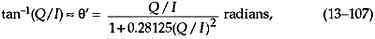
Figure 13–59 below shows the maximum error is 0.26 degrees using Eq. (13–107) when the true angle θ is within the angular range of –45 to +45 degrees. A nice feature of this θ computation is that it can be written as:

eliminating Eq. (13–107)’s Q/I division operation, at the expense of two additional multiplies.

Figure 13–59. Estimated angle theta error in degrees.
Another attribute of Eq. (13–108) is that a single multiply can be eliminated with binary right shifts. The product 0.28125Q2 is equal to (1/4+1/32)Q2, so we can implement the product by adding Q2 shifted right by two bits to Q2 shifted right by five bits.
This arctangent scheme may be useful in a digital receiver application where I2 and Q2 have been previously computed in conjunction with an AM (amplitude modulation) demodulation process or envelope detection associated with automatic gain control (AGC).
We can extend the angle range over which our approximation operates. If we break up a circle into eight 45 degree octants, with the first octant being 0 to 45 degrees, we can compute the arctangent of a complex number residing in any octant. We do this by using the rotational symmetry properties of the arc tangent:

These properties allow us to create Table 13-6 below.

Table 13–6 Octant Location versus Arctangent Expressions
So we have to check the signs of Q and I, and see if | Q | > | I |, to determine the octant location, and then use the appropriate approximation in Table 13–6. The maximum angle approximation error is 0.26 degrees for all octants.
When θ is in the 5th octant, the above algorithm will yield a θ’ that’s more positive than +π radians. If we need to keep the θ’ estimate in the range of –π to +π, we can rotate any θ residing in the 5th quadrant +π/4 radians (45 degrees), by multiplying (I +jQ) by (1 +j), placing it in the 6th octant.
That multiplication yields new real and imaginary parts defined as

Then the 5th octant θ’ is estimated using I’ and Q’ with

Information is shared by www.irvs.info